Cloning, Partitioning and formatting a new HDD

My HP laptop's HDD had been giving some errors in the Disk test for quite sometime now, so I got a new HDD with the idea to clone the old disk on this new disk. And to connect this new HDD to computer I bought a USB based 2.5 HDD External interface for HDDs, which allows you to connect the laptop disk to your system through usb cable.

My primary reason to go for cloning the disk was I wanted to avoid starting with a fresh image of Windows and the job of installing the dozens of softwares all over again. Plus I had Ubuntu installation in one of the partitions. This seemed like a perfect use-case for  disk cloning.

So, a bit of google search on disk cloning landed me on this page: https://en.wikipedia.org/wiki/Comparison_of_disk_cloning_software

I tried a couple of softwares from the above list. To keep it easy I started off with the Windows based softwares:

• Acronis True Image^[1] This one is a paid software, but luckily the new HDD I got was WD, and it turned out that if you have a WD HDD on your system, the software doesn't ask for the license and you get to use it for free. But this one turned out to be a a disappointing one as it failed to recognize my HDD as WD drive (probably because I was interfacing it through USB).
• Macrium Reflect  This was my next bet, as its a freeware with Graphical interface so going for easy one again :P. Was easy to install and then followed the GUI wizard to clone the disk, and bingo the cloning began. However as luck would have it, a couple of hours later the dialog box saying "Disk read error" popped out of no where and I was back to square one !

I realized that windows was not up to the task, the easy route was turning out to be rather difficult now.

So, I rebooted into Ubuntu this  time to try the REAL low level stuff.

• dd - is what I started with in Linux. You can create disk backups and disk cloning with a single line of this command (see thats the power of linux ;). To clone 'sda' to 'sdb' you can use the command (use at your own risk):

• dd if=/dev/sda of=/dev/sdb bs=4096 conv=notrunc,noerror

  ps -ef | grep 'dd' # get the PID of dd command

  kill -USR1 8789 #senda signal to 'dd' process to print the progress

•  WARNING: If you are thinking of trying this, please read this link, and understand what exactly you are doing because a small mistake can make you lose all your data. https://wiki.archlinux.org/index.php/Disk_Cloning
• It turned out 'dd' is just a simple copying command with no error handling built into it, so couple of hours into copying this one too failed with "input/output error" on the console :-/
• Then i tried to manually create partitions on the new disk using fdisk.

• sudo fdisk -l  #shows the disks and partition details for all disks

  sudo fdisk /dev/sdc # if you need to partition '/dev/sdc'

• The above command takes you to the fdisk command prompt, where you can easily 'create new partition', 'delete a partition' and 'write your changes to partition table' etc. However, this was turing out to be cumbersome process, because I would have to clone all partitions one by one and format them using mkfs and what not :P http://www.idevelopment.info/data/Unix/Linux/LINUX_PartitioningandFormattingSecondHardDrive_ext3.shtml
• Now comes the real awesome piece of software to my rescue - 'ddrescue'. Yeah as the name says, so it does :). This is similar to 'dd' but has disk error handling algorithm built into it. What it tries to do is recover as much of the data from the disk as is possible from the good sectors, and then uses slow reading to recover the bad sectors. You can find all the details here: http://www.gnu.org/software/ddrescue/manual/ddrescue_manual.html

• sudo ddrescue -f /dev/sda /dev/sdb logfile

  
  
• 'ddrescue' has an awesome log feature which basically logs all the disk recovery it is doing to a file. This log file allows it to resume the recovery process from where it left, incase your system crashes in between or anything !!
• You can also get a 'ddrescueview' which shows the graphical view of the recovery process as good/bad sectors etc. which is really helpful. You can download this from here: http://sourceforge.net/projects/ddrescueview/

To summarize, yeah 'ddrescue' was able to clone my old disk to the new one. And the log viewer GUI showed that my old disk had one (just one :P) bad sector in my Windows partition. But yeah, overall this turned out to be a great learning experience about disks ;)

Start a HTTP server in python

A simple HTTP Server can be started in seconds.

python -m SimpleHTTPServer

The server starts on port 8080 by default which can be changed. I have found this quite handy at times.

For example: To share a complete directory with someone over the Internet, I cd to the directory and start the server. The directory is shared, and I share my IP address. The directory can be viewed and files can be downloaded easily. I can also monitor access requests on the terminal.

original link:
http://www.quora.com/Python-programming-language-1/What-are-some-cool-Python-tricks

TopCoder SRM 567 - Div I Lvl 1

The Square Root Dilemma
-----------------------------------
=> (A*B) is the a perfect square

For a given value of (A), we try to find all possible values of B which make A*B a perfect square.

A = OA * EA,  where EA is the perfect square factor of A and OA is the other factor

So, (A*B) is perfect square when B can be factored as OA*(a perfect square).


def srm567(a,b):
    ctr = 0
    for i in range(1,a+1):
        j = 2
        s = 1
        while (j*j)<= i:
            if i%(j*j) == 0:
                s = j*j
            j += 1

        r = i/s
        #print "i,s:",i,s
        y = 1
        while (y*y*r)<=b:
            ctr+= 1
            y += 1
    return ctr

TopCoder SRM 569 - Div I Lvl 1

We need to be able to find the Operation of each bit, i.e. whether it is OR, AND , XOR.

If you see the truth table for these operations:

A	B	OR	AND	XOR
0	0	0	0	0
0	1	1	0	1
1	0	1	0	1
1	1	1	1	0

You see that the first combination where both bits A/B are '0' all the results are zero, so this combination of bits doesn't help us identify the operation. => If we have bits 0,1,1 available to be inputted at a bit position we can identify the operation.

So, now the problem reduces to finding the no. of plates to be added so that there is a combination of 011 bits available at each position.


 def srm569(plates):
    more_plates_needed = 0
    M = len(plates[0])
    for i in range(0,M):
        bits_needed = ['0','1','1']
        for j in range(0,len(plates)):
            if plates[j][i] in bits_needed:
                bits_needed.remove(plates[j][i])
        more_plates_needed = max(more_plates_needed,len(bits_needed))
    return more_plates_needed


Examples:
=======

srm569(["01010101",
 "10101010"])
Out[34]: 1

srm569(["10010101011",
 "00010101001",
 "00100010111",
 "00101010101",
 "01010111101"])
Out[35]: 1

srm569(["1101001011010",
 "0010000010101",
 "1010101011110",
 "1101010100111",
 "1011111110111"])
Out[36]: 0

Learning python regular expressions

https://developers.google.com/edu/python/regular-expressions

Python Regular Expressions

Regular expressions are a powerful language for matching text patterns. This page gives a basic introduction to regular expressions themselves sufficient for our Python exercises and shows how regular expressions work in Python. The Python "re" module provides regular expression support.

In Python a regular expression search is typically written as:

  match = re.search(pat, str)

The re.search() method takes a regular expression pattern and a string and searches for that pattern within the string. If the search is successful, search() returns a match object or None otherwise. Therefore, the search is usually immediately followed by an if-statement to test if the search succeeded, as shown in the following example which searches for the pattern 'word:' followed by a 3 letter word (details below):

str = 'an example word:cat!!'
match = re.search(r'word:\w\w\w', str)
# If-statement after search() tests if it succeeded
  if match:                      
    print 'found', match.group() ## 'found word:cat'
  else:
    print 'did not find'

The code match = re.search(pat, str) stores the search result in a variable named "match". Then the if-statement tests the match -- if true the search succeeded and match.group() is the matching text (e.g. 'word:cat'). Otherwise if the match is false (None to be more specific), then the search did not succeed, and there is no matching text.

The 'r' at the start of the pattern string designates a python "raw" string which passes through backslashes without change which is very handy for regular expressions (Java needs this feature badly!). I recommend that you always write pattern strings with the 'r' just as a habit.

Basic Patterns

The power of regular expressions is that they can specify patterns, not just fixed characters. Here are the most basic patterns which match single chars:

• a, X, 9, < -- ordinary characters just match themselves exactly. The meta-characters which do not match themselves because they have special meanings are: . ^ $ * + ? { [ ] \ | ( ) (details below)
• . (a period) -- matches any single character except newline '\n'
• \w -- (lowercase w) matches a "word" character: a letter or digit or underbar [a-zA-Z0-9_]. Note that although "word" is the mnemonic for this, it only matches a single word char, not a whole word. \W (upper case W) matches any non-word character.
• \b -- boundary between word and non-word
• \s -- (lowercase s) matches a single whitespace character -- space, newline, return, tab, form [ \n\r\t\f]. \S (upper case S) matches any non-whitespace character.
• \t, \n, \r -- tab, newline, return
• \d -- decimal digit [0-9] (some older regex utilities do not support but \d, but they all support \w and \s)
• ^ = start, $ = end -- match the start or end of the string
• \ -- inhibit the "specialness" of a character. So, for example, use \. to match a period or \\ to match a slash. If you are unsure if a character has special meaning, such as '@', you can put a slash in front of it, \@, to make sure it is treated just as a character.

Basic Examples

Joke: what do you call a pig with three eyes? piiig!

The basic rules of regular expression search for a pattern within a string are:

• The search proceeds through the string from start to end, stopping at the first match found
• All of the pattern must be matched, but not all of the string
• If match = re.search(pat, str) is successful, match is not None and in particular match.group() is the matching text

  ## Search for pattern 'iii' in string 'piiig'.
  ## All of the pattern must match, but it may appear anywhere.
  ## On success, match.group() is matched text.
  match = re.search(r'iii', 'piiig') =>  found, match.group() == "iii"
  match = re.search(r'igs', 'piiig') =>  not found, match == None

  ## . = any char but \n
  match = re.search(r'..g', 'piiig') =>  found, match.group() == "iig"

  ## \d = digit char, \w = word char
  match = re.search(r'\d\d\d', 'p123g') =>  found, match.group() == "123"
  match = re.search(r'\w\w\w', '@@abcd!!') =>  found, match.group() == "abc"

TopCoder SRM 571 - Div I Lvl 1

http://community.topcoder.com/stat?c=problem_statement&pm=12436&rd=15491
The following code prints the first 50 lexicographically sorted values of the records names:


class Test:
def __init__(self):
self.res = []
def f(self,n,x):
if x >n:
return
if len(self.res) < 50:
self.res.append(x)
#print x
else:
return

self.f(n,x*10)
rem = x%10
if rem != 9:
self.f(n,x+1)
def getRes(self,n,x):
self.f(n,x)
print self.res

Sample values printed from the program:
Test().getRes(1010,1)


1
10
100
1000
10000<
1001
10010<
1002
1003
:
1009
101
1010

TopCoder SRM 572 - Div I Lvl 1

http://community.topcoder.com/stat?c=round_overview&er=5&rd=15492


def myfunc(s,k):
    res = 0
    incr = len(s)-k
    for i in range(0,incr):
        # find the first set of alphabets which don't match
        j = i
        t = {}
        ctr = 0
        #print "i:",str(i)
        while j<len(s):
            #print "j:",str(j)
            if s[j] in t:
                t[s[j]] += 1
            else:
                t[s[j]] = 1
            j += incr
            ctr += 1
        mx = max(t.values())
        res += ctr - mx
   
    return res

TopCoder SRM 573 - Div I Lvl 1

Div II Lvl 2 problem: easier version solution
http://community.topcoder.com/stat?c=problem_statement&pm=12471&rd=15493


def myfunc(s):
    our_strength = sum(s[0:3])- min(s[0:3])
    rst = s[3:]
    #print our_strength
    if len(rst) == 0:
        return 1
    # find the rank of our team, start with rank 1 and increment it as you find better ranks
    res = 1
    rst.sort()
    #print rst
    found = True
    while found == True:
        # get the max element
        max = rst[-1]
        rst.remove(max)
        # find the min element which is greater than our_rank
        found = False
        for i in rst:
            if i+max > our_strength:
                rst.remove(i)
                found = True
                res += 1
                break
    return res

http://apps.topcoder.com/wiki/display/tc/SRM+573

TopCoder SRM 575 - DIV 1 Level 1

http://community.topcoder.com/stat?c=problem_statement&pm=12496&rd=15495

The solution for the smaller problem:


def myfunc(n):
    f = [0] *(n+1)
    for i in range(2,n+1):
        for j in range(2,i):
            if(i%j==0 and f[i-j]==0):
                f[i] =1
    print [ (i,f[i]) for i in range(0,len(f))]

The solution for the bigger problem involves getting a pattern from the above solution.
http://apps.topcoder.com/wiki/display/tc/SRM+575

Using rsync to analyse hadoop cluster logs at the name node

If you have worked on a hadoop cluster and tried going through the logs on all different cluster nodes you know how painful can it be. This script can be run on the name node and it will copy all the logs for the given hadoop job-id to the current directory of the name node. You will have to change the rsync parameters to suit yourself.

Python script:

import sys
import subprocess
import os

if len(sys.argv) < 2:
        print "Usage: python ",sys.argv[0]," <hadoop-job-id>"
        sys.exit(0)

nodes = ['192.168.112.117', '192.168.156.63', '192.168.152.31', '192.168.112.118', '192.168.156.65', '192.168.156.62' ]

#subprocess.Popen(["ls","-lr"])

for node in nodes:
        subprocess.Popen(["rsync", "-rav", "root@"+node+":/data/hadoop_logs/userlogs/"+sys.argv[1], ".")

#os.system("rsync -rav root@node-0de4bd:/data/hadoop_logs/userlogs/"+sys.argv[1]+" .")

IMP: Rsync requires that you are able to do the password-less access to these nodes from the current node (on which you are running this script.) For help on setting up password-less access check here.

Print to dynamic files from AWK cmd

To print the output of AWK to a dynamic file:

head  236_236_raw |  awk -F';' '{  print $7,"\t",$6 > ("_"$2"_"$3".txt")}'

If the number of files open are large, you will get the following error:

awk: * makes too many open files

 input record number 203, file

 source line number 1

To overcome the above problem, you can close the files like this:

head  236_236_raw |  awk -F';' '{  print $7,"\t",$6 >> ("_"$2"_"$3".txt"); close("_"$2"_"$3".txt")}'

The important point to note is that now we changed the redirection operator to ">>" from ">". Makes sense ? :)

Getting started with Facebook App development on Heroku environment

I am currently working on setting up the work environment for Facebook App development on Heroku server using python as the development language.

The complete tutorial is at: https://devcenter.heroku.com/articles/facebook

On high level the steps involve:

1. Creating a new facebook app and checking the option for Heroku hosting.
2. This creates a new domain on Heroku for your app and installs your app there.
3. Now, you can 'git clone' the code on your local machine, make changes to the code and 'git push heroku master' to push changes back to the world.
4. Need to setup the local environment for testing:
1. This involves setting up the virtualenv for python. http://www.virtualenv.org/en/latest/

virtualenv is a tool to create isolated Python environments. The basic problem being addressed is one of dependencies and versions, and indirectly permissions. Imagine you have an application that needs version 1 of LibFoo, but another application requires version 2. How can you use both these applications? If you install everything into /usr/lib/python2.7/site-packages (or whatever your platform’s standard location is), it’s easy to end up in a situation where you unintentionally upgrade an application that shouldn’t be upgraded.

Or more generally, what if you want to install an application and leave it be? If an application works, any change in its libraries or the versions of those libraries can break the application. Also, what if you can’t install packages into the global site-packages directory? For instance, on a shared host.  

In all these cases, virtualenv can help you. It creates an environment that has its own installation directories, that doesn’t share libraries with other virtualenv environments (and optionally doesn’t access the globally installed libraries either).

-----------------------------
Using Virtualenv:
http://stackoverflow.com/questions/10763440/how-to-install-python3-version-of-package-via-pip

virtualenv -p /usr/bin/python3 py3env
source py3env/bin/activate
pip install package-name

---------------------------------

Now locally test your changes before deploying on the server.

Next steps:

- https://devcenter.heroku.com/articles/python

- To be able to use Django here - https://devcenter.heroku.com/articles/django

- To be able to use a DB backend.

R, Getting Started

Download the R-package from :
http://www.r-project.org/

Download the R-studio IDE which has awesome features like auto-completion feature:

http://www.rstudio.com/

Installing a package in R (installed entropy package):
http://math.usask.ca/~longhai/software/installrpkg.html

http://math.usask.ca/~longhai/doc/others/R-tutorial.pdf

R Examples:

http://www.rexamples.com/

http://www.mayin.org/ajayshah/KB/R/index.html


-------------------------- R code to read a file into R variables -------------------

# Goal: To read in a simple data file, and look around it's contents.

# Suppose you have a file "x.data" which looks like this:
#        1997,3.1,4
#        1998,7.2,19
#        1999,1.7,2
#        2000,1.1,13
# To read it in --

A <- read.table("x.data", sep=",",
                col.names=c("year", "my1", "my2"))
nrow(A)                                 # Count the rows in A

summary(A$year)                         # The column "year" in data frame A
                                        # is accessed as A$year

A$newcol <- A$my1 + A$my2               # Makes a new column in A
newvar <- A$my1 - A$my2                 # Makes a new R object "newvar"
A$my1 <- NULL                           # Removes the column "my1"

# You might find these useful, to "look around" a dataset --
str(A)
summary(A)
library(Hmisc)          # This requires that you've installed the Hmisc package
contents(A)
describe(A)

-------------------------- R steps to load library --------------------------------------

library ('entropy') # loads the library

??entropy # shows the hep for the entropy package

Entropy calculation

http://tkhanson.net/cgit.cgi/misc.git/plain/entropy/Entropy.html

http://arxiv.org/pdf/0808.1771v2.pdf

http://vserver1.cscs.lsa.umich.edu/~crshalizi/notabene/cep-gzip.html

http://www.gzip.org/deflate.html

http://log.brandonthomson.com/2011/01/quick-python-gzip-vs-bz2-benchmark.html

http://www.gzip.org/deflate.html

Probability Theory Basics

In probability and statistics, a random variable or stochastic variable is a variable whose value is subject to variations due to chance (i.e. randomness, in a mathematical sense). As opposed to other mathematical variables, a random variable conceptually does not have a single, fixed value (even if unknown); rather, it can take on a set of possible different values, each with an associated probability.

Random variables can be classified as either discrete (i.e. it may assume any of a specified list of exact values) or as continuous (i.e. it may assume any numerical value in an interval or collection of intervals). The mathematical function describing the possible values of a random variable and their associated probabilities is known as a probability distribution.

A discrete probability distribution shall be understood as a probability distribution characterized by a probability mass function. Thus, the distribution of a random variable X is discrete, and X is then called a discrete random variable, if

as u runs through the set of all possible values of X. It follows that such a random variable can assume only a finite or countably infinite number of values.

Intuitively, a continuous random variable is the one which can take a continuous range of values — as opposed to a discrete distribution, where the set of possible values for the random variable is at mostcountable. While for a discrete distribution an event with probability zero is impossible (e.g. rolling 3½ on a standard die is impossible, and has probability zero), this is not so in the case of a continuous random variable. For example, if one measures the width of an oak leaf, the result of 3½ cm is possible, however it has probability zero because there are uncountably many other potential values even between 3 cm and 4 cm. Each of these individual outcomes has probability zero, yet the probability that the outcome will fall into the interval (3 cm, 4 cm) is nonzero. This apparent paradox is resolved by the fact that the probability that X attains some value within an infinite set, such as an interval, cannot be found by naively adding the probabilities for individual values. Formally, each value has an infinitesimally small probability, which statistically is equivalent to zero.

Formally, if X is a continuous random variable, then it has a probability density function ƒ(x), and therefore its probability of falling into a given interval, say [a, b] is given by the integral

In particular, the probability for X to take any single value a (that is a ≤ X ≤ a) is zero, because an integral with coinciding upper and lower limits is always equal to zero.

For a Random Variable, it is often enough to know what its "average value" is. This is captured by the mathematical concept of expected value of a random variable, denoted E[X], and also called the first moment. In general, E[f(X)] is not equal to f(E[X]). Once the "average value" is known, one could then ask how far from this average value the values of X typically are, a question that is answered by the variance and standard deviation of a random variable. E[X] can be viewed intuitively as an average obtained from an infinite population, the members of which are particular evaluations of X.

---------------------------------

In probability theory, the normal (or Gaussian) distribution is a continuous probability distribution, defined by the formula

The parameter μ in this formula is the mean or expectation of the distribution (and also its median and mode). The parameter σ is its standard deviation; its variance is therefore σ². A random variable with a Gaussian distribution is said to be normally distributed and is called a normal deviate.

Standard normal distribution

The simplest case of a normal distribution is known as the standard normal distribution, described by this probability density function:

The factor  in this expression ensures that the total area under the curve ϕ(x) is equal to one^[proof]. The 12 in the exponent ensures that the distribution has unit variance (and therefore also unit standard deviation). This function is symmetric around x=0, where it attains its maximum value ; and has inflection points at +1 and −1.

[edit]

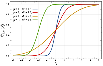
The cumulative distribution function (CDF) of a random variable is the probability of its value falling in the interval , as a function of x. The CDF of the standard normal distribution, usually denoted with the capital Greek letter  (phi), is the integral

-----------------------------

In probability theory, the central limit theorem (CLT) states that, given certain conditions, the mean of a sufficiently large number of independent random variables, each with a well-defined mean and well-defined variance, will be approximately normally distributed.^[1] The central limit theorem has a number of variants. In its common form, the random variables must be identically distributed. In variants, convergence of the mean to the normal distribution also occurs for non-identical distributions, given that they comply with certain conditions.

et {X₁, ..., X_n} be a random sample of size n—that is, a sequence of independent and identically distributed random variables drawn from distributions of expected values given by µ and finite variances given by σ². Suppose we are interested in the sample average

of these random variables. By the law of large numbers, the sample averages converge in probability and almost surely to the expected value µ as n → ∞. The classical central limit theorem describes the size and the distributional form of the stochastic fluctuations around the deterministic number µ during this convergence. More precisely, it states that as n gets larger, the distribution of the difference between the sample average S_n and its limit µ, when multiplied by the factor √n (that is √n(S_n − µ)), approximates the normal distribution with mean 0 and variance σ². For large enough n, the distribution of S_n is close to the normal distribution with mean µ and variance σ²n. The usefulness of the theorem is that the distribution of √n(S_n − µ) approaches normality regardless of the shape of the distribution of the individual X_i’s. Formally, the theorem can be stated as follows:

Lindeberg–Lévy CLT. Suppose {X₁, X₂, ...} is a sequence of i.i.d. random variables with E[X_i] = µ and Var[X_i] = σ² < ∞. Then as n approaches infinity, the random variables √n(S_n − µ) converge in distribution to a normal N(0, σ²):^[3]

---------------------------------------------

In probability theory, a random variable is said to be stable (or to have a stable distribution) if it has the property that a linear combination of twoindependent copies of the variable has the same distribution, up to location and scale parameters.

Such distributions form a four-parameter family of continuous probability distributions parametrized by location and scale parameters μ and c, respectively, and two shape parameters β and α, roughly corresponding to measures of asymmetry and concentration, respectively (see the figures).