In probability and statistics, a random variable or stochastic variable is a variable whose value is subject to variations due to chance (i.e. randomness, in a mathematical sense). As opposed to other mathematical variables, a random variable conceptually does not have a single, fixed value (even if unknown); rather, it can take on a set of possible different values, each with an associated probability.
Random variables can be classified as either discrete (i.e. it may assume any of a specified list of exact values) or as continuous (i.e. it may assume any numerical value in an interval or collection of intervals). The mathematical function describing the possible values of a random variable and their associated probabilities is known as a probability distribution.
A discrete probability distribution shall be understood as a probability distribution characterized by a probability mass function. Thus, the distribution of a random variable X is discrete, and X is then called a discrete random variable, if
as u runs through the set of all possible values of X. It follows that such a random variable can assume only a finite or countably infinite number of values.
Intuitively, a continuous random variable is the one which can take a continuous range of values — as opposed to a discrete distribution, where the set of possible values for the random variable is at mostcountable. While for a discrete distribution an event with probability zero is impossible (e.g. rolling 3½ on a standard die is impossible, and has probability zero), this is not so in the case of a continuous random variable. For example, if one measures the width of an oak leaf, the result of 3½ cm is possible, however it has probability zero because there are uncountably many other potential values even between 3 cm and 4 cm. Each of these individual outcomes has probability zero, yet the probability that the outcome will fall into the interval (3 cm, 4 cm) is nonzero. This apparent paradox is resolved by the fact that the probability that X attains some value within an infinite set, such as an interval, cannot be found by naively adding the probabilities for individual values. Formally, each value has an infinitesimally small probability, which statistically is equivalent to zero.
Formally, if X is a continuous random variable, then it has a probability density function ƒ(x), and therefore its probability of falling into a given interval, say [a, b] is given by the integral
![\Pr[a\le X\le b] = \int_a^b f(x) \, dx](http://upload.wikimedia.org/math/d/7/1/d715cf83d8a655fdfc1d3a90433cd62c.png)
In particular, the probability for X to take any single value a (that is a ≤ X ≤ a) is zero, because an integral with coinciding upper and lower limits is always equal to zero.
For a Random Variable, it is often enough to know what its "average value" is. This is captured by the mathematical concept of expected value of a random variable, denoted E[X], and also called the first moment. In general, E[f(X)] is not equal to f(E[X]). Once the "average value" is known, one could then ask how far from this average value the values of X typically are, a question that is answered by the variance and standard deviation of a random variable. E[X] can be viewed intuitively as an average obtained from an infinite population, the members of which are particular evaluations of X.
---------------------------------
In probability theory, the normal (or Gaussian) distribution is a continuous probability distribution, defined by the formula

The parameter μ in this formula is the mean or expectation of the distribution (and also its median and mode). The parameter σ is its standard deviation; its variance is therefore σ 2. A random variable with a Gaussian distribution is said to be normally distributed and is called a normal deviate.

Standard normal distribution
The simplest case of a normal distribution is known as the standard normal distribution, described by this probability density function:

The factor  in this expression ensures that the total area under the curve ϕ(x) is equal to one[proof]. The 12 in the exponent ensures that the distribution has unit variance (and therefore also unit standard deviation). This function is symmetric around x=0, where it attains its maximum value
  ; and has inflection points at +1 and −1.
in this expression ensures that the total area under the curve ϕ(x) is equal to one[proof]. The 12 in the exponent ensures that the distribution has unit variance (and therefore also unit standard deviation). This function is symmetric around x=0, where it attains its maximum value ; and has inflection points at +1 and −1.[edit]
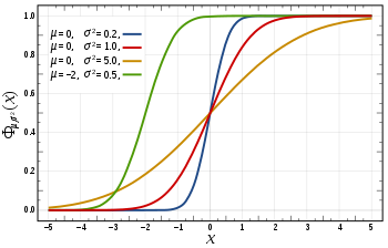
The cumulative distribution function (CDF) of a random variable is the probability of its value falling in the interval ![[-\infty, x]](http://upload.wikimedia.org/math/f/e/a/fea1695aef424e4676dafd2ddad0445d.png) , as a function of x. The CDF of the standard normal distribution, usually denoted with the capital Greek letter
, as a function of x. The CDF of the standard normal distribution, usually denoted with the capital Greek letter  (phi), is the integral
, as a function of x. The CDF of the standard normal distribution, usually denoted with the capital Greek letter (phi), is the integral
-----------------------------
In probability theory, the central limit theorem (CLT) states that, given certain conditions, the mean of a sufficiently large number of independent random variables, each with a well-defined mean and well-defined variance, will be approximately normally distributed.[1] The central limit theorem has a number of variants. In its common form, the random variables must be identically distributed. In variants, convergence of the mean to the normal distribution also occurs for non-identical distributions, given that they comply with certain conditions.
et {X1, ..., Xn} be a random sample of size n—that is, a sequence of independent and identically distributed random variables drawn from distributions of expected values given by µ and finite variances given by σ2. Suppose we are interested in the sample average
of these random variables. By the law of large numbers, the sample averages converge in probability and almost surely to the expected value µ as n → ∞. The classical central limit theorem describes the size and the distributional form of the stochastic fluctuations around the deterministic number µ during this convergence. More precisely, it states that as n gets larger, the distribution of the difference between the sample average Sn and its limit µ, when multiplied by the factor √n (that is √n(Sn − µ)), approximates the normal distribution with mean 0 and variance σ2. For large enough n, the distribution of Sn is close to the normal distribution with mean µ and variance σ2n. The usefulness of the theorem is that the distribution of √n(Sn − µ) approaches normality regardless of the shape of the distribution of the individual Xi’s. Formally, the theorem can be stated as follows:
Lindeberg–Lévy CLT. Suppose {X1, X2, ...} is a sequence of i.i.d. random variables with E[Xi] = µ and Var[Xi] = σ2 < ∞. Then as n approaches infinity, the random variables √n(Sn − µ) converge in distribution to a normal N(0, σ2):[3]

---------------------------------------------
In probability theory, a random variable is said to be stable (or to have a stable distribution) if it has the property that a linear combination of twoindependent copies of the variable has the same distribution, up to location and scale parameters.
Such distributions form a four-parameter family of continuous probability distributions parametrized by location and scale parameters μ and c, respectively, and two shape parameters β and α, roughly corresponding to measures of asymmetry and concentration, respectively (see the figures).
No comments:
Post a Comment